Teaching a Small LLM to Prefer JSON Over Prose

In my previous post, I used SFT with LoRA to teach a small model to respond in structured JSON. It worked, but SFT is imitation learning: you show the model exactly what to produce, and it copies the pattern. What if instead of demonstrating the right answer, you just tell the model which answer you prefer?

That is the idea behind RLHF, and it is how most production LLMs are aligned after pretraining. The traditional approach uses PPO with a separate reward model, which is notoriously finicky. DPO (Direct Preference Optimization) sidesteps all of that, collapsing the reward model and RL loop into a single supervised loss function.

• The RLHF Pipeline (and Why It Is Hard)
• The Bradley-Terry Preference Model
• The DPO Derivation
• DPO vs PPO
• Step-by-Step Implementation
  • 1. Generate Preference Data
  • 2. Compute Log Probabilities
  • 3. The DPO Loss
  • 4. Training Loop
• Results
  • Before and After
  • How DPO Outputs Differ from SFT
• The Implicit Reward
• When to Use DPO vs SFT
• References

The RLHF Pipeline (and Why It Is Hard)

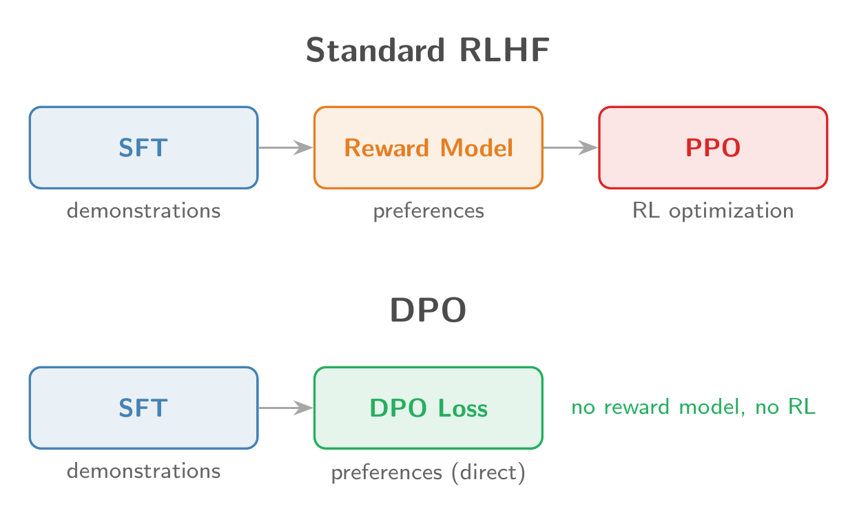
The standard RLHF pipeline has three stages:

1. SFT: fine-tune on demonstrations
2. Reward Model: train a model to score responses using human preference data
3. PPO: optimize the policy against the reward model using reinforcement learning

Stage 3 is the painful part. PPO requires generating responses (expensive), scoring them, computing advantages, and carefully managing a KL penalty to prevent reward hacking. DPO collapses stages 2 and 3 into a single supervised learning step.

The Bradley-Terry Preference Model

Both the reward model and DPO start from the same assumption. The Bradley-Terry model (1952) says: given two responses (preferred) and (dispreferred) to a prompt , the probability that a human prefers is:

where is a latent reward function. This is the same model used in Elo ratings: the probability of winning depends on the difference in strength.

In standard RLHF, you train a reward model on this, then optimize the policy against it with a KL constraint:

The DPO Derivation

The key insight from Rafailov et al. (2023): the KL-constrained problem above has a closed-form optimal policy:

Rearranging for the reward and substituting back into Bradley-Terry (the terms cancel), we get the DPO loss:

In plain English: make the model assign relatively higher probability to the preferred response (compared to the reference model), and relatively lower probability to the rejected one.

DPO vs PPO

	PPO	DPO
Models needed	3 (policy + reward + reference)	2 (policy + reference)
Training	Online RL (generate, score, update)	Offline supervised (static dataset)
Stability	Tricky (reward hacking, KL tuning)	Stable (just cross-entropy)
Compute	Heavy (generation at each step)	Light (forward passes only)

Step-by-Step Implementation

1. Generate Preference Data

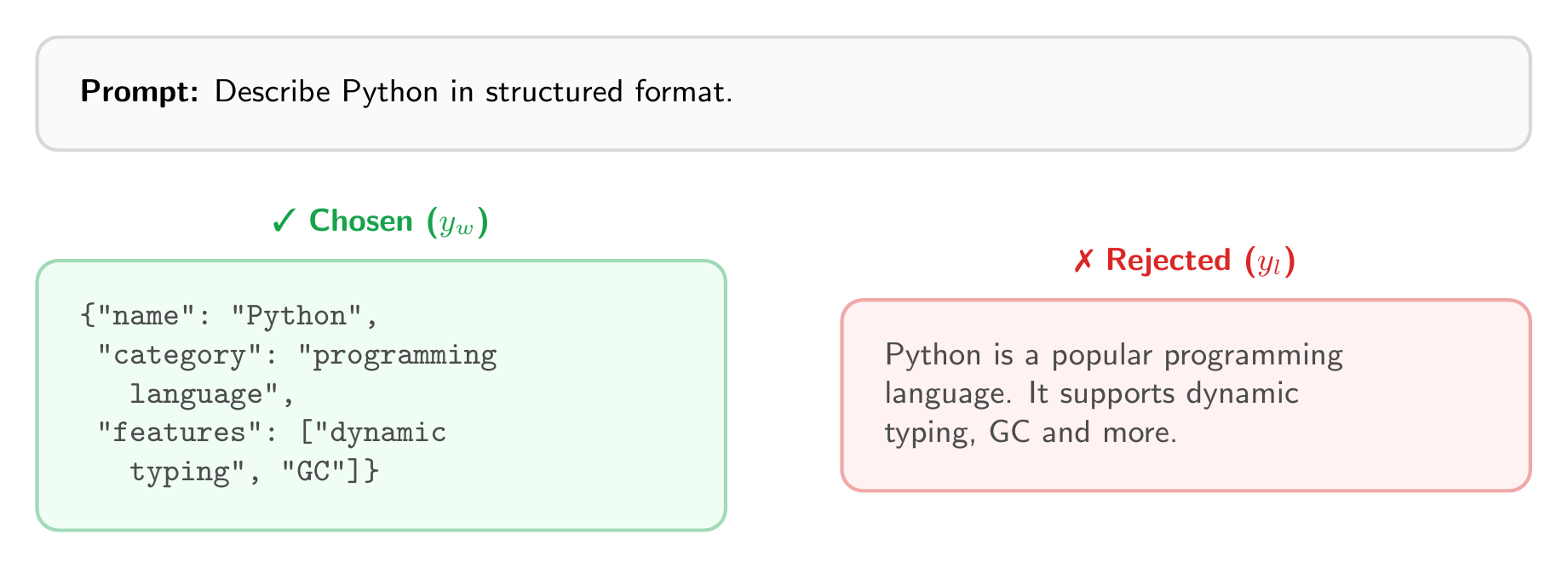
Each example needs a prompt, a preferred (chosen) response, and a dispreferred (rejected) response:

import json
import random

REJECTED_TEMPLATES = [
    "{name} is a popular {category}. It supports {feat}.",
    "{name} is a {category} known for {feat} and more.",
]

def generate_preference_data(n=500, seed=42):
    random.seed(seed)
    examples = []
    for _ in range(n):
        name, category, features = random.choice(TOPICS)
        feat = random.sample(features, k=2)
        prompt = f"### Instruction:\nDescribe {name} in structured format.\n\n### Response:\n"
        chosen = json.dumps({"name": name, "category": category, "features": feat})
        rejected = random.choice(REJECTED_TEMPLATES).format(
            name=name, category=category, feat=", ".join(feat)
        )
        examples.append({"prompt": prompt, "chosen": chosen, "rejected": rejected})
    return examples

The preference signal is clear: structured JSON is preferred over free-form text.

2. Compute Log Probabilities

The core building block. Given a model and a sequence, compute the sum of log-probabilities for the response tokens only:

import torch
import torch.nn.functional as F

def get_log_probs(model, input_ids, attention_mask, prompt_len):
    logits = model(input_ids=input_ids, attention_mask=attention_mask).logits
    log_probs = F.log_softmax(logits[:, :-1, :], dim=-1)
    target_ids = input_ids[:, 1:]
    per_token = log_probs.gather(2, target_ids.unsqueeze(2)).squeeze(2)

    # Mask out prompt tokens and padding
    response_mask = attention_mask[:, 1:].clone()
    for i in range(response_mask.shape[0]):
        response_mask[i, :prompt_len[i] - 1] = 0
    return (per_token * response_mask).sum(dim=1)

3. The DPO Loss

Remarkably short:

def dpo_loss(policy, ref_model, batch, beta=0.1):
    pi_chosen = get_log_probs(policy, batch["chosen_ids"], batch["chosen_mask"], batch["prompt_len"])
    pi_rejected = get_log_probs(policy, batch["rejected_ids"], batch["rejected_mask"], batch["prompt_len"])

    with torch.no_grad():
        ref_chosen = get_log_probs(ref_model, batch["chosen_ids"], batch["chosen_mask"], batch["prompt_len"])
        ref_rejected = get_log_probs(ref_model, batch["rejected_ids"], batch["rejected_mask"], batch["prompt_len"])

    logits = beta * ((pi_chosen - pi_rejected) - (ref_chosen - ref_rejected))
    return -F.logsigmoid(logits).mean()

That is the entire DPO algorithm. The loss pushes the policy to widen the gap between chosen and rejected log-probs, relative to what the reference model would do.

4. Training Loop

We reuse the LoRALinear and inject_lora from the SFT post:

from transformers import AutoModelForCausalLM
from sft_lora.sft.train import inject_lora  # our pure PyTorch LoRA

device = torch.device("mps" if torch.backends.mps.is_available() else "cpu")

# Reference model (frozen)
ref_model = AutoModelForCausalLM.from_pretrained(
    "TinyLlama/TinyLlama-1.1B-Chat-v1.0", dtype=torch.float32
).to(device).eval()

# Policy model with LoRA
policy = AutoModelForCausalLM.from_pretrained(
    "TinyLlama/TinyLlama-1.1B-Chat-v1.0", dtype=torch.float32
)
inject_lora(policy)  # freezes base, adds trainable A/B matrices to q_proj and v_proj
policy.to(device)

optimizer = torch.optim.AdamW(
    [p for p in policy.parameters() if p.requires_grad], lr=5e-5
)

for epoch in range(3):
    policy.train()
    total_loss = 0
    for batch in train_loader:
        batch = {k: v.to(device) for k, v in batch.items()}
        loss = dpo_loss(policy, ref_model, batch, beta=0.1)
        optimizer.zero_grad()
        loss.backward()
        optimizer.step()
        total_loss += loss.item()

    # Validation
    policy.eval()
    val_loss = 0
    with torch.no_grad():
        for batch in val_loader:
            batch = {k: v.to(device) for k, v in batch.items()}
            val_loss += dpo_loss(policy, ref_model, batch, beta=0.1).item()

    print(f"Epoch {epoch+1}  Train={total_loss/len(train_loader):.4f}  "
          f"Val={val_loss/len(val_loader):.4f}")

Note the lower learning rate compared to SFT ( vs ). DPO is more sensitive because you are optimizing a ratio of log-probabilities rather than a direct likelihood.

Results

Training TinyLlama 1.1B with DPO on 500 preference pairs (400 train / 100 val) for 3 epochs on Apple MPS:

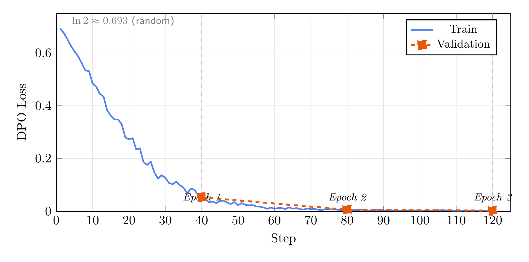
The loss starts at , which is what you get when the policy and reference model are identical (the log-ratio terms cancel, leaving ). This is a useful sanity check: if your initial loss is not near 0.693, something is wrong with your data pipeline.

By step 30 (75% through epoch 1), the model has already learned to strongly prefer JSON over free-text. Validation loss tracks closely throughout, ending at 0.003 with no sign of overfitting.

Before and After

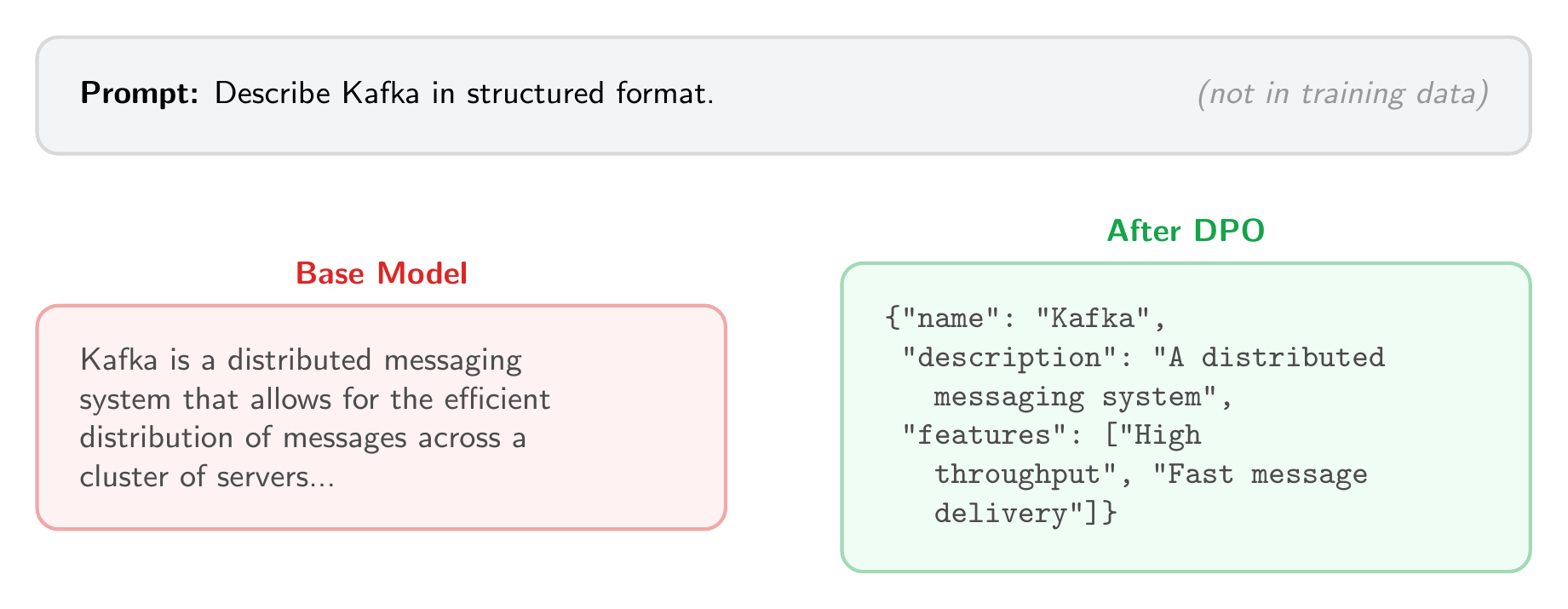
The base model interprets “structured format” as a cue for an explanatory paragraph. After DPO, the same prompt on an unseen topic yields parseable JSON.

How DPO Outputs Differ from SFT

An interesting difference emerges when you compare DPO and SFT outputs on the same prompt. The SFT model (from the previous post) produces outputs that closely match the training schema: exact field names, values drawn from the training distribution. The DPO model produces valid JSON but is more creative. It adds fields like "description" that were not in the training data, and generates feature descriptions in its own words rather than copying from the training set.

This makes sense. SFT directly maximizes the likelihood of the training outputs (imitation), while DPO only learns that JSON is preferred over free-text (preference). The DPO model has more freedom in how it satisfies that preference.

The Implicit Reward

An elegant property of DPO: even though we never trained a reward model, the policy implicitly defines one:

The reward of a response is how much more likely the trained policy thinks it is compared to the reference. In the reward modeling post, I build an explicit reward model and compare its scores to this implicit reward.

When to Use DPO vs SFT

• SFT when you have clear input/output demonstrations and want to teach a new capability
• DPO when you have preference pairs and want to steer the model toward a preferred style
• SFT then DPO is the standard pipeline: SFT teaches the behavior, DPO refines it

References

1. Rafailov, R., et al. “Direct Preference Optimization: Your Language Model is Secretly a Reward Model.” NeurIPS 2023. arXiv:2305.18290
2. Ouyang, L., et al. “Training language models to follow instructions with human feedback.” NeurIPS 2022. arXiv:2203.02155
3. Bradley, R. A. & Terry, M. E. “Rank Analysis of Incomplete Block Designs: I. The Method of Paired Comparisons.” Biometrika, 1952.
4. The full code for this post is available at github.com/mrrostam/blog-code/dpo