How LLM Quantization Actually Works
I got interested in quantization from two directions. At work, I spent time inside picoLLM‘s inference engine, digging into how its compression algorithm squeezes models down for on-device deployment. Outside of work, every time a new local model drops, I find myself staring at a list of GGUF variants on Ollama or llama.cpp trying to pick between Q4_K_M, Q5_K_S, Q8_0, and wondering what I am actually trading off. This post is what I have learned about quantization through those experiences.
- The Basics: What Quantization Does
- The Outlier Problem
- Post-Training Quantization (PTQ) vs. Quantization-Aware Training (QAT)
- GPTQ: Second-Order Optimization
- AWQ: Protecting Salient Weights
- GGUF: The CPU-First Format
- SmoothQuant: Taming Activations
- The Frontier: Sub-4-Bit and 1-Bit
- Choosing a Method
- References
The Basics: What Quantization Does
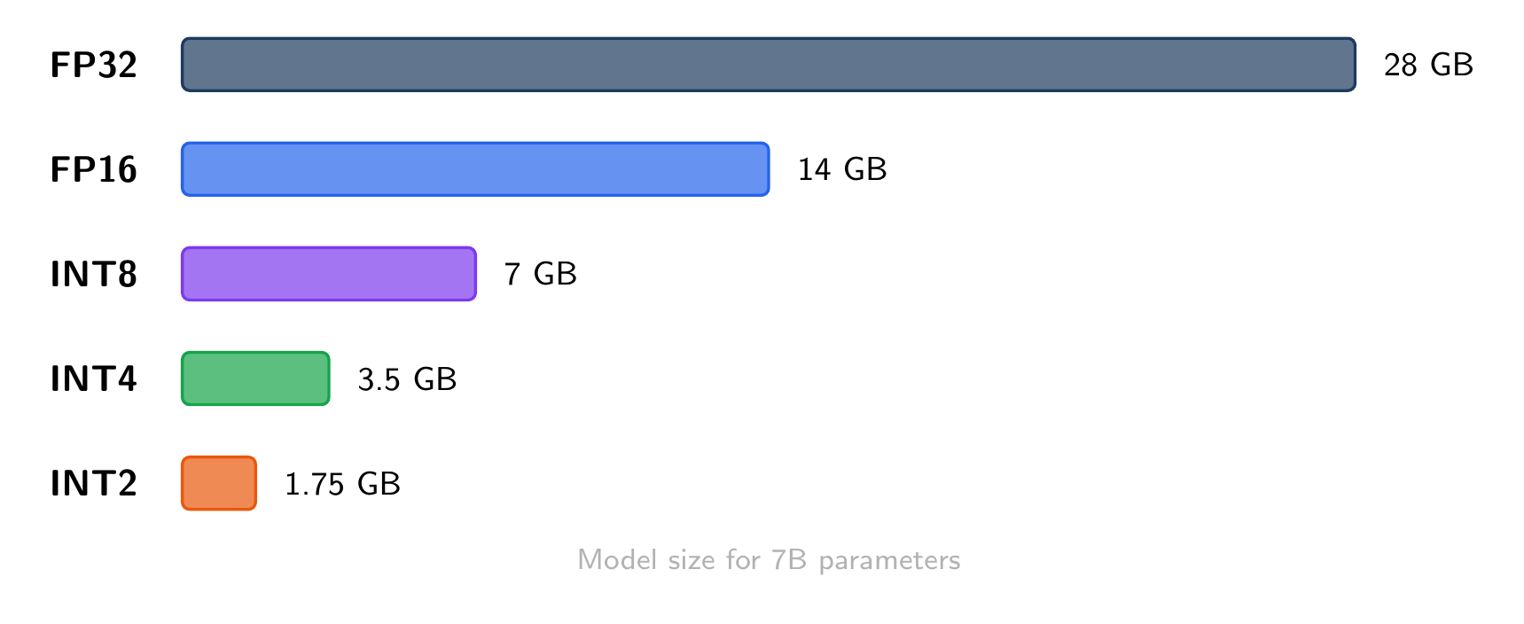
Neural network weights are stored as floating-point numbers, typically float16 (16 bits each). Quantization maps these to a smaller set of values using fewer bits:
The core operation is simple. To quantize a float value
where
Symmetric vs. Asymmetric
Symmetric quantization sets
Asymmetric quantization uses a non-zero
Most LLM weight quantization uses symmetric, because transformer weights are roughly centered around zero.
Per-Tensor vs. Per-Channel vs. Per-Group
The granularity of the scale factor matters a lot:
- Per-tensor: one scale for the entire weight matrix. Fast but coarse.
- Per-channel: one scale per output channel (row). Much better accuracy, standard for INT8.
- Per-group: one scale per group of
consecutive weights (e.g., ). The sweet spot for INT4, used by GPTQ and AWQ.
Finer granularity means more scale factors to store (overhead), but less quantization error per weight.
The Outlier Problem
Here is why naive quantization fails on LLMs. Transformer activations contain outlier channels: a small number of hidden dimensions with values 10-100x larger than the rest. If you set the quantization range to cover these outliers, the vast majority of “normal” values get crushed into a few quantization bins, destroying information.
This was first documented by Dettmers et al. (2022) in the LLM.int8() paper. Their solution: decompose the matrix multiplication into two parts. The outlier dimensions (about 0.1% of channels) stay in float16, while everything else gets quantized to INT8. This mixed-precision decomposition is what makes INT8 quantization work for LLMs without quality loss.
Post-Training Quantization (PTQ) vs. Quantization-Aware Training (QAT)
PTQ takes a trained model and converts weights to lower precision after the fact. No retraining needed. All the methods below (GPTQ, AWQ, GGUF) are PTQ.
QAT simulates quantization during training, inserting fake-quantize operations in the forward pass so the model learns to be robust to rounding. Better quality at very low bit-widths, but requires the full training pipeline. QLoRA is a notable example: it trains LoRA adapters on top of a 4-bit quantized base model.
For deployment, PTQ is the standard path. You quantize once and serve.
GPTQ: Second-Order Optimization
GPTQ (Frantar et al., 2022) treats quantization as an optimization problem. Instead of rounding each weight independently, it asks: given that I am going to round this weight, how should I adjust the remaining weights to minimize the overall output error?
The algorithm builds on Optimal Brain Quantizer (OBQ), which processes weights one at a time. For each weight
where
GPTQ’s key innovations over OBQ:
- Quantize in arbitrary order (columns, not one weight at a time), enabling batched processing
- Lazy batch updates: accumulate corrections and apply them in blocks of 128 columns
- Cholesky decomposition for numerical stability when inverting the Hessian
The result: GPTQ can quantize a 175B parameter model to 4 bits in about 4 GPU-hours, with negligible perplexity increase. It is the most widely used method for GPU-based INT4 inference.
When to use GPTQ: GPU inference, 4-bit or 3-bit, when you want the best accuracy at a given bit-width and have a GPU for the one-time quantization step.
AWQ: Protecting Salient Weights
AWQ (Lin et al., 2023) takes a different approach. Instead of optimizing the quantization of every weight, it focuses on protecting the ones that matter most.
The key observation: only about 1% of weights are “salient” (important for model quality), and you can identify them by looking at the activation magnitudes. Weights connected to high-activation channels have an outsized impact on the output. Quantizing these carelessly causes disproportionate error.
AWQ’s solution is elegant. Instead of keeping salient weights in higher precision (which would require mixed-precision hardware), it applies a per-channel scaling before quantization:
where
The optimal scale
When to use AWQ: GPU inference, 4-bit, when you want fast quantization (faster than GPTQ) with comparable quality. AWQ is also more robust to different calibration data.
GGUF: The CPU-First Format
GGUF is not a single quantization algorithm but a file format and ecosystem built around llama.cpp. It supports a family of quantization types optimized for CPU inference.
Decoding the Names
When you see a GGUF quant type like Q4_K_M, each part means something:
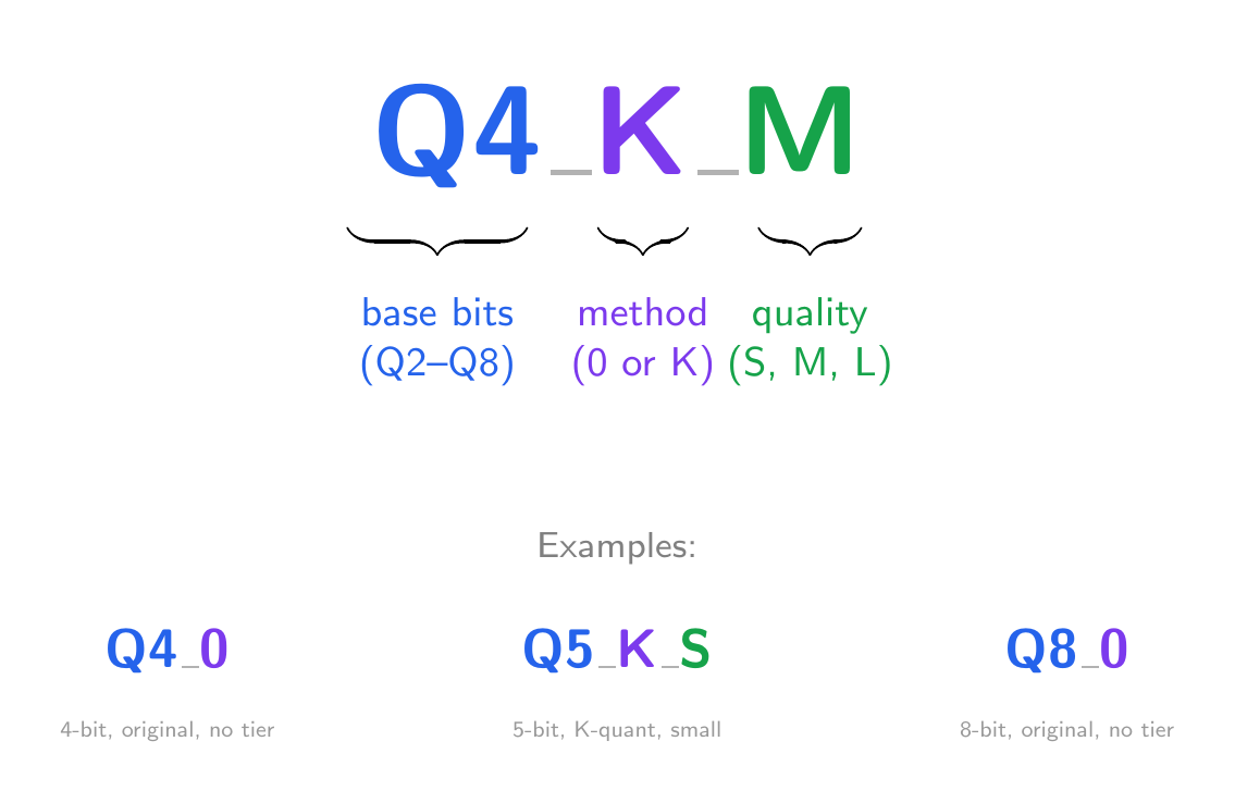
The first part is the base bit-width: Q2 through Q8, the number of bits used for the majority of weights.
The middle part is the method:
- No suffix (Q4_0, Q8_0): the original “type-0” scheme. Each block of 32 weights gets one shared FP16 scale factor
. Quantization is symmetric: , dequantization is . Simple and fast, but forces the range to be symmetric around zero. - K (Q4_K, Q5_K): “K-quant”. Each block stores both a scale
and a minimum , enabling asymmetric quantization: , dequantization is . This captures the actual range of each block more tightly. K-quants also use importance-based mixed precision: attention layers get more bits than feed-forward layers within the same file.
The last part is the quality tier (K-quants only), controlling how aggressively the mixed-precision allocation compresses different layers:
- S: more layers get the lower bit-width, smallest file
- M: balanced allocation, the default choice
- L: more layers get the higher bit-width, best quality
Common Types
| Type | Avg bits/weight | 7B model size | Quality |
|---|---|---|---|
| Q8_0 | 8.5 | ~7.7 GB | Near-lossless |
| Q6_K | 6.6 | ~5.5 GB | Excellent |
| Q5_K_M | 5.7 | ~4.8 GB | Very good |
| Q4_K_M | 4.8 | ~4.1 GB | Good (most popular) |
| Q4_0 | 4.5 | ~3.8 GB | Decent |
| Q3_K_M | 3.9 | ~3.3 GB | Acceptable |
| Q2_K | 3.4 | ~2.8 GB | Noticeable degradation |
The “avg bits/weight” is higher than the base number because of the overhead from storing scale factors and minimums per block.
Why K-Quants Win
The key insight behind K-quants is that not all layers are equally important. In a transformer, the attention projection weights (Q, K, V, O) have a larger impact on output quality than the feed-forward layers. K-quants exploit this by assigning different quantization types to different layers within the same file. A Q4_K_M file might use Q6_K for attention layers and Q4_K for feed-forward layers, averaging out to about 4.8 bits per weight.
GGUF’s strength is the inference runtime. llama.cpp uses hand-optimized SIMD kernels for dequantization during matrix multiplication, making CPU inference surprisingly fast. It also supports partial GPU offloading: keep some layers on GPU, the rest on CPU.
When to use GGUF: CPU or mixed CPU/GPU inference, laptops, Ollama/llama.cpp deployment. Q4_K_M is the most popular balance of size and quality. If you have the RAM, Q5_K_M or Q6_K are noticeably better.
SmoothQuant: Taming Activations
The methods above quantize weights only. SmoothQuant (Xiao et al., 2022) tackles the harder problem of quantizing both weights and activations to INT8 (W8A8).
The challenge is the outlier problem described earlier. SmoothQuant’s insight: migrate the quantization difficulty from activations (hard, because of outliers) to weights (easy, because they are fixed and well-behaved). It does this with a per-channel scaling:
The scale
After smoothing, both
When to use SmoothQuant: server deployment with INT8 hardware support, when you want to quantize both weights and activations for maximum throughput.
The Frontier: Sub-4-Bit and 1-Bit
QuIP# and AQLM (2-bit)
At 2 bits per weight, standard methods break down. QuIP# (Tseng et al., 2024) and AQLM (Egiazarian et al., 2024) push into this regime using more sophisticated techniques:
- QuIP# uses Hadamard rotations to spread outlier information across all weights (making them “incoherent”), then applies lattice codebooks for efficient 2-bit encoding.
- AQLM uses additive multi-codebook quantization: each group of weights is represented as a sum of entries from learned codebooks, optimized end-to-end.
Both achieve usable quality at 2 bits, which was previously considered impossible for LLMs. A 70B model at 2 bits fits in about 17GB, runnable on a single consumer GPU.
BitNet b1.58 (1.58-bit)
BitNet b1.58 (Ma et al., 2024) goes further: every weight is ternary, taking values from {-1, 0, +1}. This is not post-training quantization but a fundamentally different training recipe. The model is trained from scratch with ternary weights.
The “1.58 bits” comes from information theory:
This is still a research direction. You cannot take an existing model and convert it to 1.58 bits. But it suggests that future models may be trained natively in low precision.
Choosing a Method
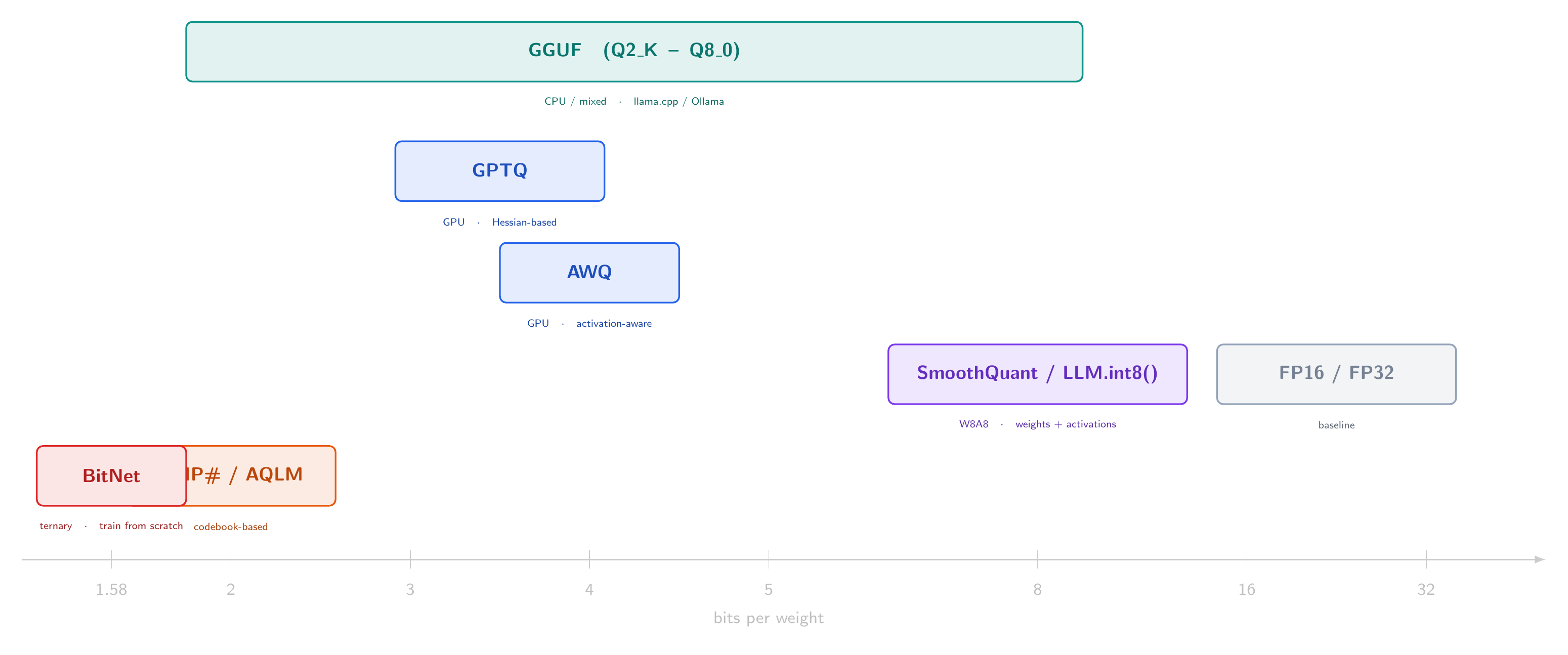
| Method | Bits | Target | Quantizes | Speed |
|---|---|---|---|---|
| GPTQ | 3-4 | GPU | Weights | Slow (hours) |
| AWQ | 4 | GPU | Weights | Fast (minutes) |
| GGUF (K-quant) | 2-8 | CPU/GPU | Weights | Fast |
| SmoothQuant | 8 | GPU (INT8 HW) | Weights + activations | Fast |
| LLM.int8() | 8 | GPU | Weights + activations | Fast |
| QuIP# / AQLM | 2 | GPU | Weights | Slow |
| BitNet | 1.58 | Custom HW | Trained natively | N/A |
For most people deploying small LLMs locally: GGUF Q4_K_M through Ollama or llama.cpp. For GPU serving: AWQ or GPTQ at 4 bits. For maximum throughput on INT8 hardware: SmoothQuant.
References
- Frantar, E., et al. “GPTQ: Accurate Post-Training Quantization for Generative Pre-trained Transformers.” ICLR 2023. arXiv:2210.17323
- Lin, J., et al. “AWQ: Activation-aware Weight Quantization for LLM Compression and Acceleration.” MLSys 2024. arXiv:2306.00978
- Xiao, G., et al. “SmoothQuant: Accurate and Efficient Post-Training Quantization for Large Language Models.” ICML 2023. arXiv:2211.10438
- Dettmers, T., et al. “LLM.int8(): 8-bit Matrix Multiplication for Transformers at Scale.” NeurIPS 2022. arXiv:2208.07339
- Dettmers, T., et al. “QLoRA: Efficient Finetuning of Quantized Language Models.” NeurIPS 2023. arXiv:2305.14314
- Tseng, A., et al. “QuIP#: Even Better LLM Quantization with Hadamard Incoherence and Lattice Codebooks.” ICML 2024. arXiv:2402.04396
- Egiazarian, V., et al. “Extreme Compression of Large Language Models via Additive Quantization.” ICML 2024. arXiv:2401.06118
- Ma, S., et al. “The Era of 1-bit LLMs: All Large Language Models are in 1.58 Bits.” 2024. arXiv:2402.17764